

What is linear regression in simple terms?
Linear regression in simple terms is a supervised learning algorithm that uses the relationship between data points to form a best fit line called a regression line.
If there is a strong relationship in the data then the regression line is used to calculate the value of a variable, the target variable, based on one or more features.
For example, if there is a relationship between the weight of an item and the price then we can use regression line to predict the item price based on weight.

In this article we use simple examples to explain linear regression including correlation, prediction, and evaluation.
The performance of linear regression is reliant on the strength of relationship, or correlation of the data. It is possible to measure the correlation using a metric such as Pearson’s correlation.
Given correlation, the regression line should be the ‘line of best fit’ to the data. There are several metrics used to either create, measure, or evaluate this line. The most common approach is explained as the ‘sum of least squares’, sometimes referred to as ‘ordinary least squares (OLS)’.
The two evaluation metrics that show how good a fit the regression line is, and therefore an indicator to how the performance of linear regression can be applied on the dataset are ‘r squared’ and the ‘root mean square error (RMSE)’.
These metrics are confusing to a beginner as there are also metrics called ‘r’, mean squared error (MSE)’, and mean absolute error (MAE)’.
This article will explain all these important aspects of linear regression with the use of orange, a simple tool used for machine learning.
We will start off with simple linear regression and assume a strong relationship between two variables.
Simple Linear Regression Prediction
Lets take a sequence of numbers and try to predict the next number in the sequence. Here is the sequence of numbers:
4 8 12 16 20 24 28 32 36 ?
Easy yes? The answer is below the chart if you need to check.
Now you have made a guess we can look at the sequence of numbers in a chart. We can predict the value of the next number by following the line.

When our line meets the tenth number (10) on the horizontal axis (x-axis) then it will have the value seen in the vertical axis (y-axis). So the next number is of course 40. Lets try another example.
2.6 6.4 8.6 12.4 14.6 18.4 20.6 24.4 26.6
What is the next number in the sequence? Lets look at the sequence of numbers in a chart.

This is similar in that the numbers are increasing by 3 rather than 4 therefore the answer is about 30, but there is a difference in this example.
We can see the numbers increasing by 6 every two examples, either from 2.6 to 8.6, 14.6, 20.6 and 26.6, or from 6.4 to 12.4, 18.4 and 24.4. Therefore we know the next number will be 24.4 + 6 which is 30.4.
Given a set of values we can predict a future value based on an average of the relationship if there is a relationship, or ‘correlation’. So, for example, if your salary increases by a percentage each year you can forecast what it will be in 1 year, 2 years or even 10 years time.
This is the basis of linear regression.
Regression is a measure of relationship (like year to salary increase), and linear is similar to a straight line. So we can think of linear regression as modeling the line that shows a relationship.
We can then use a value and make a prediction by seeing where it crosses this line, like the tenth value in our list, or year equals ten for the salary increase.
Regression Line
Given a set of data points, we can draw a line showing the relationship of these points. As we know from our studies in mathematics, we can define a line by using the formula:
y = mx + c
where m is the line slope and c is the place where the line crosses the y-axis called the y intercept. The slope is also called the coefficient.
There is also another version of the formula with e for error:
y = mx + c + e
Ordinary least squares (OLS)
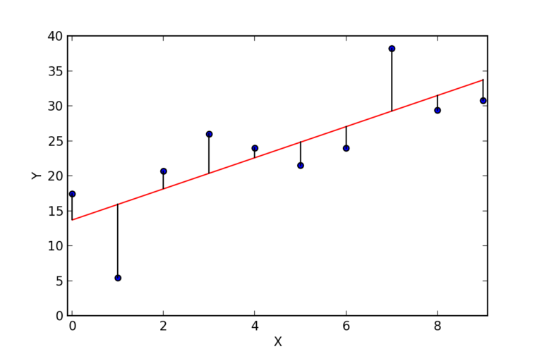
So how do you calculate the regression line? To identify the line of best fit we can use a method based on the least difference from the points to a potential regression line.
If we draw a line from each point to a line separating the data points we can measure the difference from the line and the data (see image above). These line are called residuals.
To decide if the line is the ‘best fit’ we can take each difference from the data points to the line, the residual, and square the figure to remove the positive / negative aspect. The sum of these squares then gives us a score.
We can try a different line and calculate the sum of squares. The least sum of squares indicates the better fit. We can continue this with many potential lines to find the least sum of squares, although we can a program to calculate the linear regression line for us.
Linear Regression Correlation
So far we have assumed a strong relationship between two variables. This relationship, or correlation, can be measured.
A common metric to measure is the Pearson correlation.
Pearson's Correlation
The Pearson correlation metric measures the linear relationship between two variables with a score of 0 given for lack of any relationship, a highest score of 1 for a positive correlation and a lowest score of -1 for a negative correlation.
We can see the three levels of correlation in orange. The first example shows the value of the variable of the y-axis increasing when the x variable increases, giving a rising regression line.

In the orange widget for correlation the Pearson correlation score is 0.916.

The second example shows a random selection of data points with little to no correlation. The low Pearson correlation score is -0.086.

The third example shows the value of the variable of the y-axis decreasing when the x variable increases, giving a regression line going diagonally downwards.
The Pearson correlation score is -0.951.

Multiple Regression
In multivariate linear regression, or multiple regression, there are more independent x variables.
For example, if we wanted to calculate the price of a house, we would need t o use a range of factors, called features, such as house size, land size, location, number of bedrooms and bathrooms etc.
Linea Regression Terms
regression
Regression is the relationship between two variables, a dependent variable and one or more independent variables.
In machine learning there is supervised and unsupervised learning. supervised learning is either regression or classification.
In this case we consider regression as a measure that is a continuous number (e.g. student % mark, 80%), as opposed to classification (e.g. student grade, ‘A’).
linear regression
Linear regression in simple terms is a supervised learning algorithm that uses the relationship between data points to form a best fit line called a regression line.
independent / dependent variables
Having the linear regression line allows us to see the relationship between the two variables, or how the dependent variable (house size) affects the independent variable (house price).
coefficient
The coefficient in linear regression is the slope. If the regression line is y=3x + 5 then the coefficient is 3.
intercept
The intercept in linear regression is the place where the regression line meets the y-axis.. If the regression line is y=3x + 5 then the intercept is 5.
line of best fit
The linear regression line is the best fit line to the data points. Linear regression uses a line that is the best fit to the data to make predictions.
To calculate the line of best fit we can measure the distance between the line and the data points. The least distance from potential regression lines and the data points indicates the best fit.
residuals
The line from the regression line and the data points.

sum of least squares
The sum of least squares is the measure of the total lengths of the residuals squared.
The best fit line will have the least total when the residuals are measured from the line, squared, and added together.
ordinary least squares (OLS)
The sum of least squares
R
A measure of the relationship between two variables with a value between -1 for a negative correlation, and +1 for a positive correlation.
A dataset with no correlation will have an R score of 0.
R squared
A measure of the variance from the mean to the regression line. R squared has a value between 0 and 1. A high R squared score indicates a line of good fit.
Video Data files
In the video called Linear Regression Evaluation | Analysis using Orange we use two data files. These are csv files and are available for download here: